Executive Summary link HERE

Like Artificial Sweeteners, Artificial Intelligence comes in many forms and flavors. And AI will be as incorporated into our daily lives as Splenda. But can the current incarnation of Machine Learning result in a conscious super-intelligence? One that may present an existential threat to humanity? To dig deep into what's possible I built a simple Neural Network (NN) and put it through its paces. The results were surprising.

Much of AI relies on marketing hype. The term "neural network" gives the impression that computers have developed biological brains that "learn" and even "hallucinate." Since we still don't understand how consciousness emerges from our own biological brains, not understanding the "black box" of an artificial neural network can lead us to believe that artificial consciousness may also emerge.

Artificial Neurons, Really?

Called "Perceptrons" before the AI Winter of the 1970s, the rebranded "neural networks" used today are still assembled from basic, easy-to-understand math. Think of the artificial neurons as Lego blocks that are connected from an "Input Layer" through one or more "Hidden Layers" to finally an "Output Layer." It's one big math function assembled from simple pieces. Artificial neurons are a cartoonish model of real biological neurons. They are way too simple. But they have some similarities which makes them useful, and the analogy is tempting.

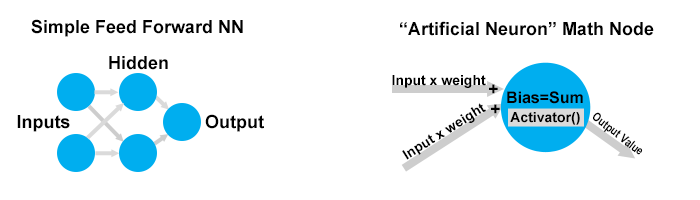
You read the diagram above from left to right. Grey arrows direct the flow of values from one operational node to the next. "Inputs" have a single value entered into them. The "Hidden" and "Output" nodes sum multiple input values and basically share the same structure.

Typically Inputs take values from the real world and the Output is a summary decision about that data.

What these nodes have in common with the model of a biological neuron is as follows: Each "neuron" has one-to-many inputs with a variable value for each. The neuron has it's own bias which is applied to each input. The values of input + bias are summed inside the neuron. When a threshold is reached, a biological neuron will "fire," creating the input for the other neurons to which it's connected. It always has the same intensity but will vary its frequency rate. With artificial neurons, the resulting value is always passed along at the same pace, after passing through the activator function (which is like the threshold mechanism in a cell). So having one-to-many inputs, summing the inputs, and using a threshold to determine what to output, that is how artificial neurons are similar to real ones.

So far the math part of this is trivial and would not seem to create unexplainable reasoning coming from a "mysterious black box." The inputs are real numbers, they are multiplied by real number "weights" and added to a real number "bias". These products are then summed up in each node. Just simple multiplication and addition.

Here's an example: Input A is 100 and its weight is 1. Input B is 50 and its weight is 2. The node bias is 5. So 100(1)+5 =105 and 50(2)+5= 105. Summed, the internal value is 210. The sum of 210 is passed through an Activator function for that node (just one Activator per node, like the bias). The Activator can be the more sophisticated part of math. We will come back to it in a moment.

Weights and Biases are Essential for Learning

That there are various inputs and outputs as part of the decision-making network seems obvious. The use of a weight for each input gives the system the ability to find the right level of importance for each component input. When an artificial neural network is "learning" it is finding the appropriate value, or importance, of each input by adjusting weight values up or down. The bias serves the same purpose but is a fixed offset instead of a skew.

The process of feeding example data into the neural network and adjusting the weights and bias values to get a desired output is called "training." When the weights and biases attain a set of "optimal values" then no more "learning" takes place and the network's purpose shifts to pure decision-making.

The Simplest Function

In grade school, I would usually cringe when math assignments involved "functions," e.g. f(x)=2x + 5. They look like equations but teachers couldn't explain to me why they were different. It wasn't until a graduate course in Game Theory that my professor offhandedly said, "And of course, a function is just a way to map one value to another." Unbelievable.

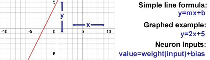
So the inputs to the neurons are just simple line formulas that could be individually graphed. If there are multiple inputs their values are just added together. The weight can be 1 to just pass a value forward, >1 to amplify it, 0 to ignore it, a decimal like 0.5 to divide the value's input or it can even be negative. The weights provide the full complement of grade school math: Addition, Subtraction, Multiplication, Division.

The Universal Approximation Theorem

When solving business problems I have not previously utilized NN as a technique. Instead, I have worked directly on creating functions that map business processes. As an example, I created a "Price Optimizer" for an e-commerce site. Inputs included price, source and level of inventory, assortment completeness, a time series weighted average of past sales, etc. The formulas were much more sophisticated than y=mx+b and contained variables that I then used the computer to optimize over time. So I am comfortable utilizing explicit functions (instead of many "math nodes") and "iterative optimization" (instead of bulk "training").

In a nutshell, the Universal Approximation Theorem (circa 1990) says an Artificial Neural Network of sufficient size and complexity can approximate any mathematical function.

My thinking was that after I built a functioning neural network (NN) from scratch, I would be able to "simplify the equations" and end up with a single comprehensive function. There are a lot of online tutorials for building neural networks, but all seem to involve downloading Python libraries and then just trusting the output. One I liked, Introduction To Neural Networks by Victor Zhou, also utilizes the Python language. However, the author explained enough of his math that I could recreate the project in another programming environment and compare it against his results.

Activation Functions

The "activation function" portion of an artificial neuron's math is like the "action potential threshold" of a biological neuron. There are many choices between activation functions for a single node and an artificial neural network might utilize several. A simplistic example might be "If the summed value is positive then output 1, otherwise output 0."

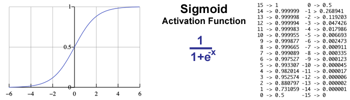
Don't freak out over the math behind the Sigmoid function. Like the simplistic example, its purpose is to push values to either 1 or 0. (You will see why very soon.) An input value of 6 or higher results in almost 1.0, and at 15 and anything above it is 1.0. The opposite happens with negative values mapping toward 0. An input value of 0 results in an output of 0.5, which represents maximum uncertainty between 1 and 0.

Sex is Binary

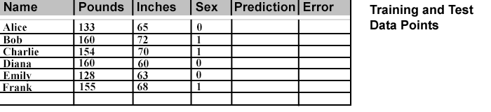
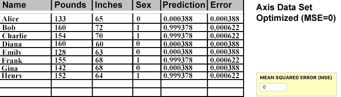
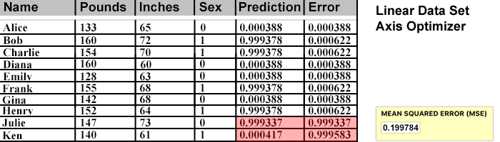
We are ready to start looking at the artificial neural network (NN) I built, extending the example of Victor Zhou. Victor selected a tiny fictional set of males and females, with data points named "Alice", "Bob", "Charlie", and "Diana." He trained his NN and then added two more "test" data points named "Emily" and "Frank." His system reaches an accuracy of about 0.04 on his test subjects.

With an accuracy goal to match or beat, there were a few changes I made to Victor's data points. First, I assigned females to 0 and males to 1, because the input data is higher for the males and the math seems easier if the output values don't have to cross over. Second, Victor subtracted a pseudo average from the Pounds (body weight) and Inches (height) values outside of the NN input node. This gives negative values for the female values and positive for the males. I instead incorporated that math into a hidden layer so I could easily add more inch and pound values directly.

An Accurate Stereotype was not my Goal

The purpose here is to build a neural network (NN), understand the deterministic math behind it, and then see if I could distill the optimally trained network into a single function.

I wanted to duplicate a "Black Box" and then crack into it.

Of course, the values for the males and females in the data set are only kind of representative, and in reality, sex is not determined or predicted by height and weight measurements. There are also solid counter-examples, but the result would be a trained model with inherently lower accuracy. I wanted to see if I could get perfect accuracy that matched a specific function, i.e. all predicted males fall on one side of a line, while all the females fall on the other side.

Non-Random Optimization

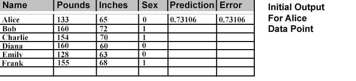
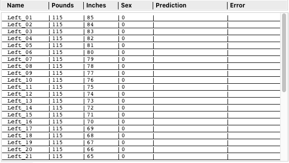
Here's more of what happens during a Training Phase. (And for my purpose, everything was the training phase.) You have a data point, like Alice's pre-determined Categorization (Sex) value which is a 0. Alice's two input values, 113 for Pounds, and 65 for Inches (see table above) are entered into the two Input nodes, and the values "Feed Forward" through each connected neuron until an Output value emerges from the end. This Output value is the "Prediction" and it is matched against the Categorization value to determine the "Error." A perfect prediction has an error of 0.

To determine the overall accuracy of the trained NN, you square the error values for each data point and take that average. It's called MSE (mean square error) and the squaring makes every error a positive number (so positive and negative error values don't cancel out) and it also emphasizes larger errors.

You could set weights and biases indiscriminately high to make every prediction come up 1. That would create great predictions for the male examples, but be terrible for the females.

So you need to test the prediction error for all the data points, and the data set needs to properly represent all the possible categories. (This last point is critical to the discussion of why AIs make biased decisions).

The common way to optimize the weight and bias values is to use a combination of calculus and randomization called "stochastic gradient descent." The calculus indicates where the error is diminishing, and the randomization tries to prevent it from getting stuck at a false minimum.

Since Vince provided a solid example of using calculus to optimize for this data set, and the result (0.04) I decided to try another approach. If I could not significantly improve on the 4% error, I would default to the calculus-based technique.

However, I don't like the trend of deifying randomness and brute force. Faster computers have encouraged this, as has distributed computing. Cloud providers LOVE this approach. Splitting up a problem across thousands of rented processors is the way they get rich. New software engineers frequently assume this is the natural, and only way, to solve tough problems.

I had success solving Traveling Salesman Problems (TSP) with a few techniques that might apply. The NN and TSP situations are similar in this way: The TSP presents a series of locations and the goal is to arrange a path that minimizes the overall distance of a round trip. Optimizing an NN involves finding the set of weights and biases that minimize the error between each data point's prediction and its categorization. Minimizing overall distance between points, and minimizing overall error between predictions, tempted me to use a common approach.

Graphic User Interface

Writing self-contained desktop applications has somehow fallen out of favor. But if I intended to break into the black box I wanted an in-depth visual interface. Let's take a look at the application I wrote:

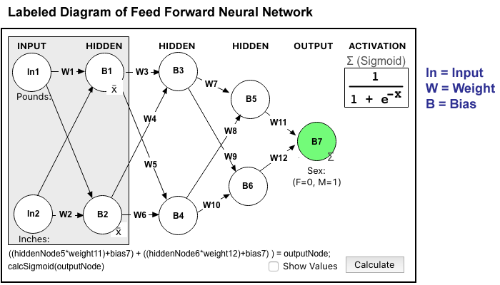
The diagram above represents the design of my NN. The arrows show how the values flow from Input to Output. The grey box indicates the nodes and weights that are "given" for each data point (like Alice) and the rest of the weights are used for optimization. The goal of this NN is to take an input of Pounds and Inches and output a number close to 0 or 1. A human pre-assigned the category of 0 or 1 to each data point (again, think Alice), and the NN mathematically makes a prediction trying to match it.

Initial Values

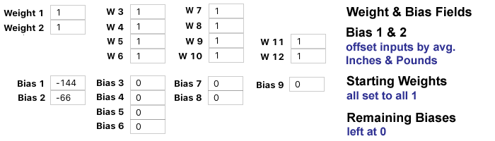
The Ws on the diagram arrows are for the numerical Weights. To simplify the math I left all the Bias values at 0 and just optimized Weights. If you assign all 0s to the Weights, the Output will be 0.5 for every data point because of the Sigmoid Activation (remember 0 maps to 0.5 in the Sigmoid diagram above.) So a decent starting value is all 1s for the weights.

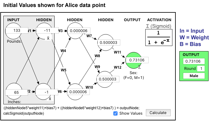
The above Values are revealed at each node for the Alice data point. The two inputs are specific to Alice and the calculations are based on the Weighting of 1 and the Sigmoid Activation. The final Output value of 0.73106 is a very poor prediction and would categorize Alice as a 1 (Male) which is the opposite of the desired prediction.

Record Predictions and Errors

The output Prediction for Alice is recorded in the data table. The difference between the "Sex" value and the Prediction is recorded as the Error for that data point.

Before any adjustments to the weights, every data point is input and the resulting Prediction and Error are recorded. Then the MSE is calculated for the total Error for that set of Weights. This MSE is the number we will use to evaluate whether the accuracy of a different set of weights results in a better or worse predictive model.

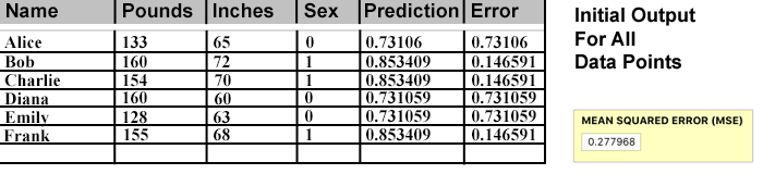
A bigger MSE value is worse. The MSE for all weights at 1 here is 0.277968. For reference, if we started with all weights at 0, each data point would be an indeterminate 0.5 (Sigmoid effect placing the output exactly half-way between 1 and 0). The MSE for those data points would be 0.25. Conclusion: The all 1s weight set is even worse than all 0s! And it's because of the highly erroneous Male prediction (0.73) for the Female data points.

We Have Some Work To Do

We could try to manually guess the optimal value of each weight individually, but it wouldn't work. The values can be literally any number, positive or negative, including fractional values. To tackle the potential complexity, I included drop downs in the interface to set Max and Min values and the steps between them. A bit of trial in error demonstrated that values above 10 and below -10 didn't help, (mainly because the Sigmoid Function clips off extremes and pushes toward 1 and zero). Since we are using a computer, and I drastically minimized the number of selections, you might think we should just brute force every potential combination and compare MSEs. However, with 10 weight fields (W3-W12) and 21 potential values (-10 through 10), there would be 21¹⁰ (or 16,679,880,978,201) full MSEs to compare. So no Brute Force.

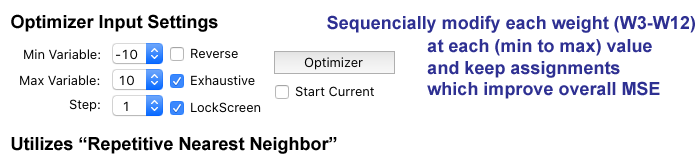
The Nearest Neighbor algorithm comes from the Traveling Salesman solution tool set. You start with a first location and then just pick the next location that's closest. Continue until you have strung all the locations together. It's fast but frequently the final location added is really far away and does not result in the optimal path. The overall distance is also high dependent on which location is the start. "Repetitive Nearest Neighbor" gives a much better result, because it runs once with each of the locations as the new start. The overall distances are compared for each start and the shortest path is the eventual solution. It takes longer because it has to run once for every location, but not the gazillion brute force combination of every location.

The Algorithm Succeeds!

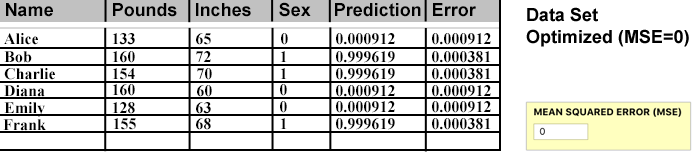
My goal was to beat the 0.04 error rate of Victor's example project. You can see below the Predictions definitely outperformed the standard (calculus + randomization) method. MSE for our data set, carried out 6 decimal points, is ZERO.

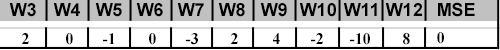
Weight Combinations and MSE

Below you can see a condensed history of attempted weight values and their MSE. The top line is all 1s and as the algorithm made successive improvements the MSE continued to improve.

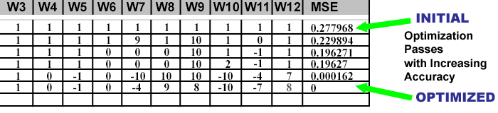
The last line achieves an MSE of 0 and optimization is considered complete.

But what a crazy set of values that created this optimal result!

Even though we have thoroughly gone through all of the simple math components that make up this NN, how the optimization process was able to reach a solution with these values is unclear. At this stage, it really is a "Black Box" after all.

If the Universal Approximation Theorem is correct, there should be some matching mathematical function that would represent this result in a simpler and more understandable way. What can be used to help reveal the implicit function?

Lines are for Graphing

My next step would be to look at the data graphically to check for a pattern. I manually typed the values into the Desmos Graphing Calculator and something became apparent.

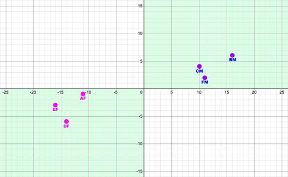
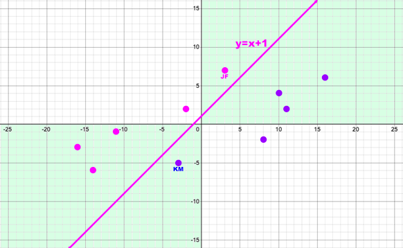
I added color and labels to keep track of the individual points. Alice is the pink dot at (-11,-1) labeled "AF" (for "Alice-Female")

What I noticed was the data points were already pre-assigned in a nice split, with all the Males in the positive quadrant and the Females in the negative one. The Quadrants happened when the input values were subtracted from the overall averages. Females went to negative values and Males to positive, and the Sigmoid pushed negative numbers to 0 and positive numbers to 1. So the implicit solution doesn't need a linear function, just an IF statement about positive or negative values.

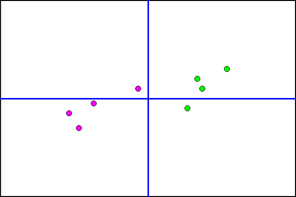
Using a Function to Drive Data

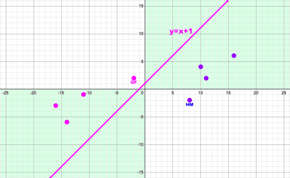
I put a line on the graph and then added two more data points (GF and HM) that would invalidate the IF statement approach, but be correctly predicted if the NN found the solution of the line. I wanted to test the Universal Approximation Theorem: Can the NN really find this function?

Two New Data Points

Gina and Henry are added to the Training Data Table and the Optimization runs again successfully.

However, with new data added, the set of optimal weights is different from before...

The NN finds an optimal solution, but is it using an equivalent to y=x+1 like in my Desmos graph? How would I be able to tell?

Time for a Custom Graphing Module

The pretty Desmos graph is a web application, but not integrated with my NN program. To get to the bottom of what is happening I created a rudimentary graph module that takes values from the Training Data Table directly. This will turn out to be key.

I changed the color of the Male data points to green so they contrast better. Comparing to the Desmos graph I can see all the placements are spot on.

My impression is that the clean way to separate the two groups would be a nice line that looks like y=x+1. But how many data points would it take to confirm that's what's happening? Do I keep adding more fictional Male and Female points are see if they can be optimized?

Birth of Neural Network CT Scan

In a flash of inspiration, I created an entirely new set of data points for the Training Table. I labeled them "Left_01" through "Left_39." On my graph, the far left (x-axis) data point is equivalent to 115 Pounds. From top to bottom (y-axis) the Inches run from 85 down to 47. So I created 39 replacement data points and assigned all their categories as 0 (Female).

The graph of these new data points looks like this:

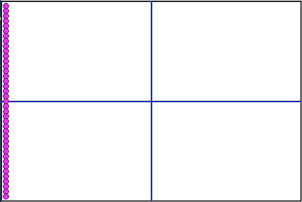
Instead of running the Optimizer against this set of data points to get the optimum set of weights, I ran each individual data point against the existing Optimized weights. If the Error was 0.01 or less, I added an additional 1 Pound to that data point (eg "Left_01") and ran it through the NN again. I kept incrementing the Pounds value and checking the Error unit it exceeded 0.01. Then I moved the point back one step to get the last value as it's Max. Next, I moved down to the next data point (eg "Left_02") and maximized its Pounds, and repeated until all points had marched across the graph to the right. That scanning technique should reveal the boundary line (function) of what was being predicted as Female (0).

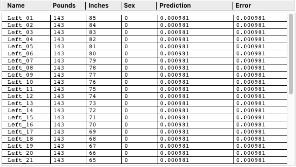
At first, I thought I made a programming error. The values went from all being 115 Pounds to all being 143 Pounds. But when I graphed the scan, it became apparent the NN was doing something different from what I expected.

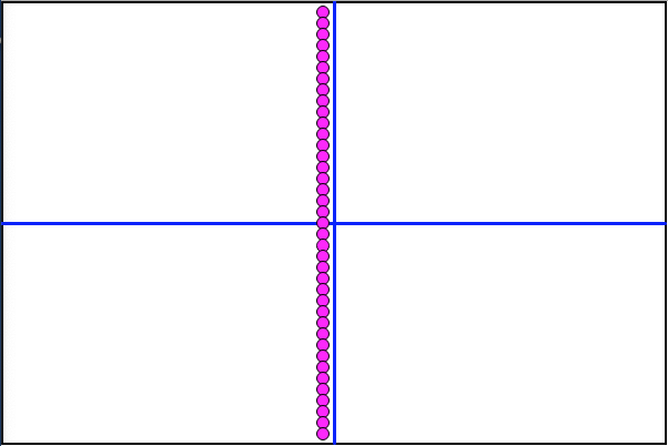
Instead of using a function y=x+1 like I was anticipating, it found a simpler solution, the y-axis itself!

To see if the NN could find a more sophisticated function, I would have to give it more of a challenging data set. I checked my Desmos graph to find some new values: JF and KM. These are two additional data points that cross the axis and should require re-optimization.

Before optimizing for this expanded data set, I checked against the existing "Axis Optimizer" weights. The two new data points received opposite predictions and dragged down the MSE significantly.

A fresh run of the Optimizer against this new Training Table data results in a great MSE again, although the smallest bit less accurate (.0000001 vs 0.0)

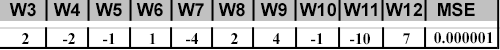
Each individual error is slightly higher than before, despite many efforts. It seems to be as good as it will get.

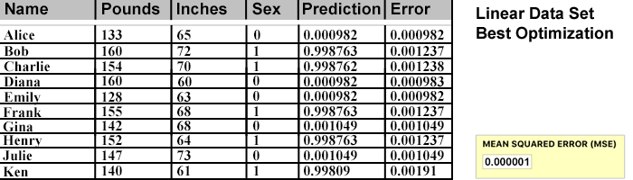
With new Optimal Weights for this data set, it's time to run the CT Scan and graph the results. Will the NN have approximated y=x+1 as intended?

BINGO!

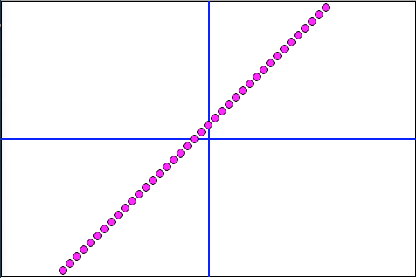
Desmos graphed a line using the formula y=x+1 (see previous). But nowhere in the NN or its explicit programming does that function exist. Instead, the line of dots (directly above) is the result of a set of NN-Weighted values, optimized for the individual points from Training Table data. Each dot moved one at a time, scanning across the optimization grid.

What Have We Learned So Far?

Primary Conclusions:

• The set of Optimized Values for an Artificial Neural Network continues to render it a Black Box.
• The Novel CT Scan method created here provides graphic, human-readable results.
• We finally have a visual demonstration supporting the Universal Approximation Theorem.
• There exists an implicit function that drives the predictions of a trained NN.
• The predictive function of an NN may not align with human intelligence expectations.
• Even a few new points of data can drastically shift the implicit function, driving the predictions of an NN.

What's Next?

PART TWO will tackle the challenge of a non-linear function. That is, if the data requires more sophisticated delineation than provided by a straight line, can the NN find it? Will changes to my current NN architecture need enhancement to tackle this?

PART TWO »