Previously on Black Boxes...

In Part One we went through the design of a simple Feed Forward Neural Network (NN).

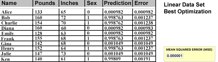
We loaded a minimal set of Training Data and set a goal of an MSE (Mean Square Error) rate of 0.000000 after Optimization. Then we began to look at the data graphically to see if some kind of mathematical function could be hidden in the behavior of the NN.

That a function might be found is predicted by the Universal Approximation Theorem.

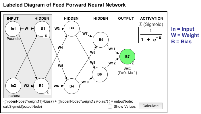
The output of Nodes labeled with B3 through B7 all use the Sigmoid Activation, pushing values toward 1 or 0. Nodes B1 and B2 just subtract the average and pass values forward.

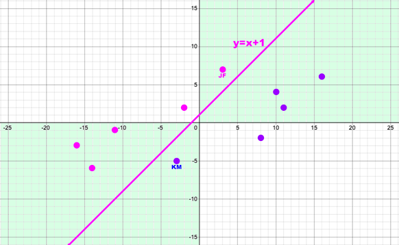
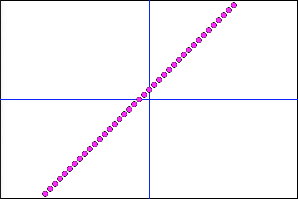
Desmos Visualizes Where New Data Could be Placed

Looking at a graph of the data points and plotting a line (linear function) shows where to place new data points. The new points are used to force the NN to re-optimize from its current implicit strategy.

New data points are added to the Training Table data and the Optimization program is run until a new acceptable MSE value is achieved.

With new Optimal Weights for this data set, it's time to run the CT Scan and graph the results. Will the NN have approximated y=x+1 as intended?

The CT Scan Reveals an Implicit Linear Function

Astonishingly, the CT Scan Graph matches the intended Desmos line function perfectly.

The Scan above is checking the left boundary data points (Females) by increasing the Pounds value until the Error rate becomes greater than 0.01.

Time for Enhancements!

The first order of business is to expand the CT Scan to include data points coming in from the Males (M). Prior to the Scan, data points line up at far left (F) and far right (M).

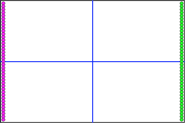
After the Scan, points butt up against either side of the implied linear function.

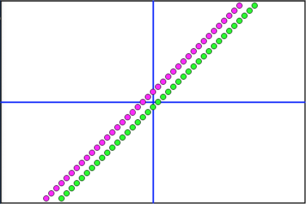
The conclusion here is that the NN being used can, in fact, approximate a linear function (eg y=x+1) if challenged with the right data.

A Much Harder Challenge

Expanding on the current data set, can we force the NN to find a more difficult type of function? A quadratic has a form like y=x² + 3x - 6. The problem with x² is that it results in a horseshoe shape on the graph that doesn't fit with the current data set. But what about a trickier cubic function? This will have the x value cubed (x³) and create an S-shape on the graph instead of being a simple straight line.

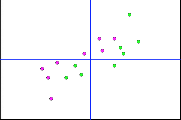
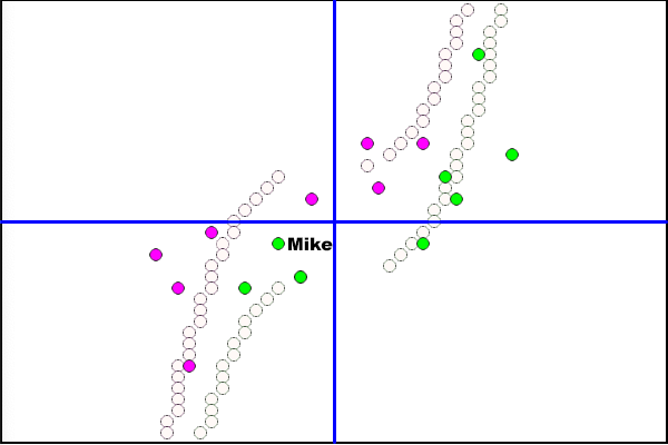
Desmos Shows Where New Data Points Can Fit

I engineered a cubic function I thought would wind through the existing data points and yet be easy to track. "0.008x³" is 0.2x times 0.2x times 0.2x. So the increment of the optimizer would need 0.2 as a step when trying different weights instead of the previous step of 1.

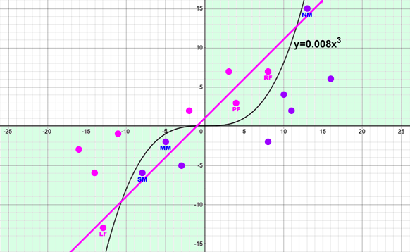
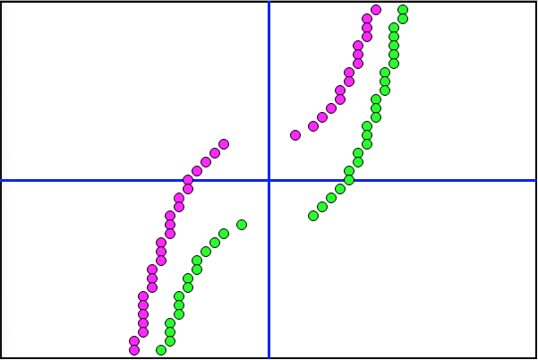
The above graph shows where 6 new data points would be inserted: 3 new Male assignments (NM, MM, SM) and 3 Female (RF, PF, LF). They are intentionally placed so that any quadrant, axis, or straight-line-based solution will mis-predict them. To achieve an optimal MSE score, a cubic function will have to be approximated by the NN.

Enhanced Direct Formula Check

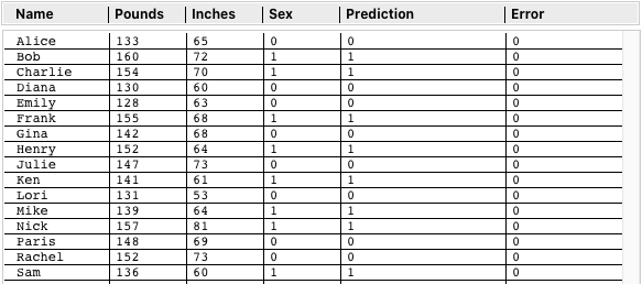
Below are All 16 Data Points Used for the Cubic Function Challenge.

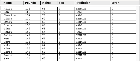
Instead of using the NN and Optimization to numerically predict the Sex value (0 or 1), I created a button to run the data for each against the formula y=0.008x³. The Prediction column contains "FEMALE" or "MALE" based on which side of the line they fall on. It's not a test yet of the NN, but rather a confirmation that the data does really conform to the function shown on the Desmos graph.

Without any lines to guide your eye, think about threading through these new data points.

Activation Function Conundrum

The current NN architecture can't begin to achieve acceptable optimization with this data. The best MSE is about 0.135. Even a CT Scan won't run since any point has to be more accurate than 0.01 to be plotted.

The problem lies with the choice of Activation Functions. Previously I passed a value straight through or pushed it to 1 or 0 with the Sigmoid function. No matter how many more hidden nodes are added, the NN won't do x³. Because nodes SUM the values arriving, the NN could do x+x+x but not x*x*x. Multiplication is handled by the weight assignments, but a particular weight does not vary between all the data values running through the node.

So the answer is a "custom" activation function. Instead of the trickier math that scales a value toward 1 or 0, just x³ the input. While we are at it, another node with x² and one with a pass though (just x) might allow the NN to use or ignore various nodes and approximate a sophisticated function like y=2x³ + x² + 3x - 6.

The New (Cubic) Design

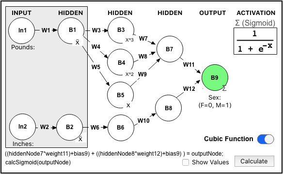
First notice there is a "Cubic Function" toggle in the screenshot. This lets me switch between the new cubic and previous linear designs to better understand their effects. It also explains the spacing between the rows in the screenshot of the original. (It makes room for the two additional nodes (B4 and B5).

I also eliminated all the extra cross-over connections as the weight values would be zero and just create unnecessary calculations during optimization. It's called "trimming."

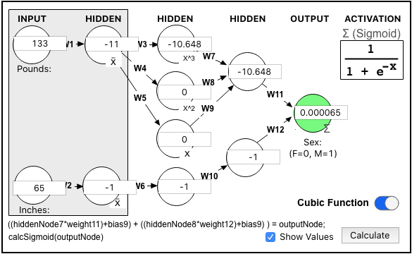
The Sigmoid Activation is still present at B9 since we ultimately still want a predicted output of 1 or 0. B1 and B2 still use their Biases to subtract the values from the average, yielding positive and negative input values. B3 has a x³ Activator, B4 has x², and B5 is just a pass-through of x. B6, B7, and B8 are also pass-throughs and rely on the weights and input summing as before.

Manually Assigned Solution

Previously I demonstrated that taking the input values and using a straight math function, instead of running the NN calculations, gave 100% correct Predictions (but without any precision.) This is the table above showing 16 "MALE" and "FEMALE" Predictions for y=.008x³.

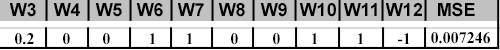
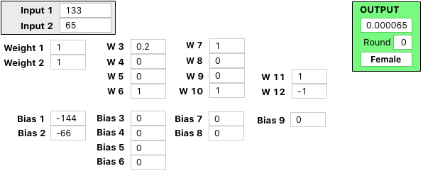
The structure of this NN should mean I can manually assign the weights (instead of running the Optimizer) yet recreate the math of y=0.008x³. The weight assignments to recreate this are extremely simple:

Here is the NN Diagram showing all the interim values for the "Alice" data point:

Here are the full Weights and Biases, so you can follow the math if you'd like...

Here are the results for the entire Training Table data points:

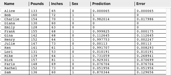
Alice has a very good accuracy rate of 0.000065; and Bob, Diana, and Emily are dead on. In fact, all of the Predictions are correct, but some are not so confident. A standout is Mike with an error of 0.268941. The total MSE for the set is 0.007246. Acceptable, but not matching the 0.000000 results from Linear Optimizations. It seems like an exact manual weight assignment would represent the case of best accuracy.

CT Scan Says...

Running the full Scan against this Training Set yields the following interesting graph.

My intuition says since the boundaries of the dotted lines are set at an error of 0.01 or less, the data points with higher error rates (like Mike) should fall in between.

An Image Overlay and We Have Our Confirmation

The Mike data point does fall the farthest from its (right) boundary. The error rates and distance from the CT Scan boundaries correspond throughout.

Final and Most Surprising Outcome

Having manually forced the weight values to duplicate the exact formula used with Desmos seemed like it would define the upper bound of accuracy. However, I gave the NN and chance to run its own Optimization and was honestly shocked at the result.

The Error Rates are ZERO Across the Board!

What kind of weights did the NN come up with during Optimization?

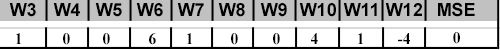
The first observation is that the x value is increased from 0.2 to 1. The y value is also increased at three stages, totaling 96 times. That would make the effective formula 96y=x³. Let's see what the CT Scan looks like:

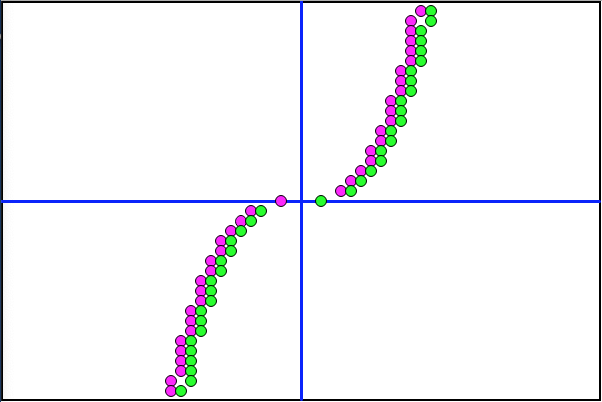
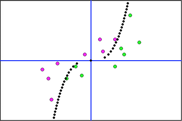
Wow. Super tight!

Lastly, let's plot the 16 data points and implied function (96y=x³), then make sure everyone ends up on the correct side of the line.

Optimized is Optimal

The NN was challenged to find a function for manipulated data requiring a cubic solution. It was stunningly successful.

Final Conclusions

• The Universal Approximation Theorem creates a link between normal mathematical functions and the mind of an Artificial Neural Network (NN).
• The CT Scan method provides further insight into the behavior of the NN.
• A neural network can be trimmed and supplied with exponential Activators, enabling it to find solutions requiring sophisticated implied functions.
• The implied function that drives an NN's predictions can be drastically shifted with the planned addition of very few data points.
• Startling results can emerge from a small NN with a small number of data points. They do not require big data, randomization, or brute force. The magic is in the math.
• The power of a Neural Network comes from finding a mathematical function that optimally matches the data.

HOME »

You can leave thoughtful comments or questions at the link below.

Comments   ?