ARCHIE and the Automata
The Emergence of Complexity
May, 2026
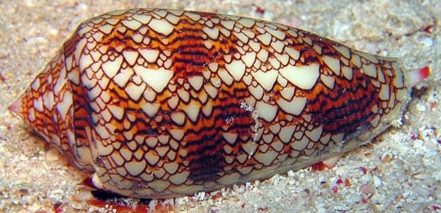
The 20th Century saw many of the greatest minds attempt to map biological structures to simple mathematical formulas. Turing (1952) linked iterative calculation to patterns on animal shells and hides. Ulam and von Neumann (1949) used Cellular Automata (CA) to help explain self-replication. And Ulam (1962) expanded the CA model to speculate about the developing morphology of plants.

In the 1980s, Mathematica inventor Stephen Wolfram took the study of CAs to a new level with his introduction of Elementary Cellular Automata (ECAs)1.
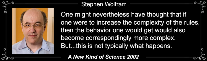
"I made what at first seemed like a small discovery: a computer experiment of mine showed something I did not expect. But the more I investigated, the more I realized that what I had seen was the beginning of a crack in the very foundations of existing science, and a first clue towards a whole new kind of science."
—Stephen Wolfram, "A New Kind of Science", 2002
Welcome to the Neighborhood
Wolfram's contribution was to simplify Cellular Automata to the point where the particular ECA model could be exhaustively studied.
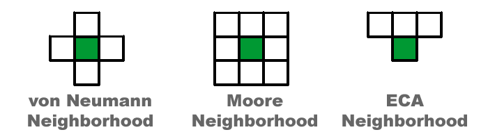
Von Neumann's model only considered cells that were "adjacent", meaning they shared a side. In the language of Cellular Automata, the cells around the target are considered its "neighborhood." For ARCHIE to detect Objects against a background, all the pixels touching the target pixel must be considered. For CAs, this would be equivalent to the "Moore Neighborhood.1" For Wolfram's Elementary Neighborhood, only the cells immediately above are considered relevant, since ECAs only build downward.
The number of possible states ARCHIE has to consider for each target pixel is substantial. Since there are 10 possible colors for each pixel and 8 pixels surrounding the target, there are 108 (100,000,000) potential states to evaluate for just a single pixel.
Popular CA models are normally limited to two states (or colors). This cuts down the possible states tremendously. The ECA Neighborhood has only 3 input cells, so there can be only 8 possible ways to influence each downstream cell.
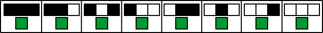
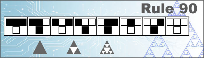
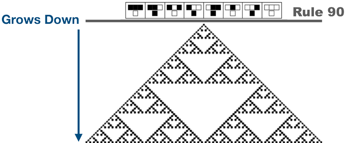
The illustration above shows how an ECA "Rule" appears. One difference in practice is that the target green cells will have either a black or white designation. The top row of triple boxes represents eight possible configurations for a cell. Taken together, the set of all eight makes up a single named "Rule." Noticing there are only two output states for each of the triplet configurations, Wolfram named the Rule for the counting number of its binary interpretation.
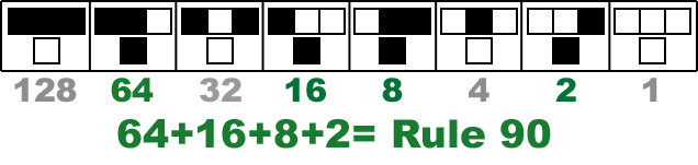
Wolfram's naming scheme means ALL possible rule sets will take names from "Rule 0" to "Rule 255." If you know the name, you can easily translate this to an ECA configuration.
Programming Your ECA
Here are the basics...
Each different ECA Rule specifies how the next row of cells will be populated. You get to pick the starting cells in row 1, the number of columns wide, and how many rows down to process. In the animation above, Rule 4 only has a single segment, which produces a cell. Only when the cell directly above is populated does a cell "live" to the next row. Both upper corners must also be empty. The result is a line of cells straight downward.
Rule 2 is another single-segment program. The cell below will always shift one to the left. I started the illustration with 3 live cells so you could see multiple cells being affected.
All of the segments in the ECA Rule template have a mirrored segment. They have either left-to-right mirror or a black-to-white mirror. The mirror of Rule 2 is the single active segment in Rule 16. If I made a similar animation, all of the live cells would shift right on the next row.
More than the Sum of Its Parts
Since the segment for 2 produces a left diagonal, and the segment for 16 produces a right diagonal, you can expect that combining both segments into Rule 18 would produce a simple pyramid-like triangle. But something additional happens.
The first three rows proceed as expected, but the 4th row begins to show an internal structure. This is the first point at which segments 2 and 16 start interacting, and not merely growing based on their own live cells. The more "generations" applied as rows, the more involved the structure becomes:


Rule 18 (left) after 26 generations. Despite fewer active segments than Rule 90 (right), the end patterns are identical when beginning with a single live cell. That seems like another surprising outcome.
Sensitive to Initial Conditions
Both Rule 18 and Rule 90 have active segments 16 and 2. Those are solely responsible for the patterns above. Rule 90 additionally has mirror segments 64 and 8. Under the condition of a centered cell starting cell, segments 64 & 8 are somehow never activated.
However, if we begin with random cell assignments on the top line, the differences in these two rules become more apparent:

These two detailed illustrations from the excellent Elementary Cellular Automata" at atlas.wolfram.com
Rule 90 yields a darker pattern because it produces more detailed structures. There are some embedded triangles that echo an iteration of its fractal basis, but are strangely mutated instead.


Magnified portions from above for Rule 18 (left) and Rule 90 (right)
reveal their differences, triggered under initial random conditions.
The takeaway is that different ECA Rules can produce patterns that mirror one another, or produce identical results when starting from the same basic conditions, and then differ wildly when the initial conditions are changed.
Rule 90 and the Sierpiński Triangle
One of the simplest fractals is known as the Sierpiński Triangle, Sierpiński Sieve, or Sierpiński Gasket. It was first documented by Polish mathematician Waclaw Sierpiński in 1915. Some are quick to point out that some mosaics, as far back as the 11th century, exhibit the property of recursively divided triangles.
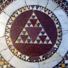
11th-century Mosaic with Triangle Motif
The difference between the recursive mathematical definition and the mosaic implementations is that the mosaics typically stop after 4 iterations and begin inserting triangles elsewhere. Stonework follows its own set of restrictions, and the goals are decorative rather than mathematical.

Divide each side of a black triangle at the midpoint and cut away the new, smaller triangle.
The geometric version of Sierpiński's triangle involves recursively dividing each resulting figure further inward. With Rule 90, the Cellular Automata proceeds DOWNWARD, row by row, and somehow anticipates the same Fractal Geometry as the INWARDLY DIVIDING process.
Tower of Sierpiński
This article is part of the series about ARCHIE, the classic AI application I wrote to solve ARC Prize problems. How ARCHIE works is explained in detail in my article "ARCHIE." The ARC Prize was always oriented toward probabilistic LLM tools, but after the contest pivoted to ARC-2 and ARC-3 puzzles, I decided we had parted ways on what was important to discover. Instead, I chose to advance ARCHIE's capabilities on Classic AI problems, including "Blocks World." These are problems considered beyond the capability of modern approaches.
The second article in the series is "Illusion of Thinking," in which ARCHIE tackles the famous Tower of Hanoi problem. Something I discovered while working on this article is that the "Tower of Hanoi" and the "Sierpinski Triangle" are related. Let's briefly check that out.
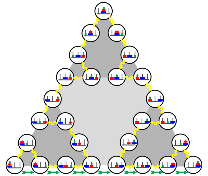 The Green Arrow path is the most efficient 'Tower of Hanoi' solution and was followed by ARCHIE. Yellow shows an alternate rule in which disks move only to adjacent pegs. This requires visiting every possible state.
The three-disk version of the Tower problem reveals the basic Sierpinski triangle above. Adding more disks adds more states and more iterations to the graph. As the disk number grows, the fractal nature becomes ever more apparent.
ECAs and the ARC Puzzle Format
If ARCHIE can solve the Tower of Hanoi puzzle, can it detect and decipher a Rule 90 puzzle? Can an ECA be represented in the ARC puzzle format, and would a human problem solver see the solution as obvious?
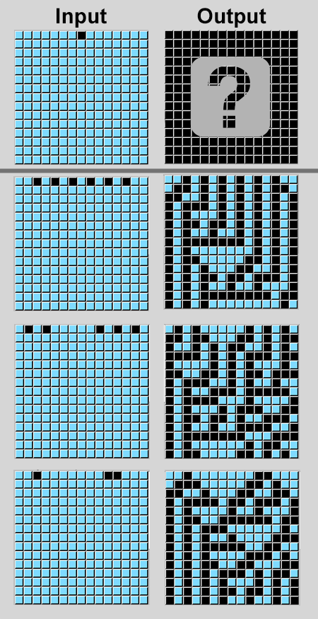
As a refresher, ARCHIE's representation of an ARC puzzle has the top inputs/outputs row as the question to be answered. The next three rows are example inputs/outputs to help you formulate a rule. You apply the rule to the test input, which replaces the blank output grid.
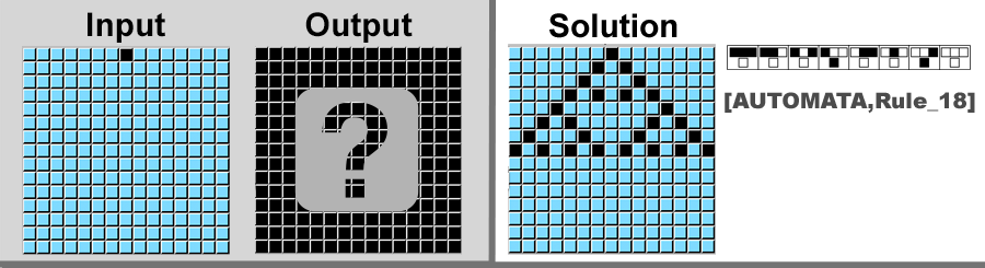
If we look at the first example row, we notice the output seems to be an extension downward of any black pixel from the input. Looking at the second example, the theory seems to hold. The last example breaks that pattern, however. The two adjacent black pixels don't extend at all. What sort of rule is this?
Since the input doesn't include any adjacent pixels, I would create an output solution of a single column of black pixels extending to the bottom. And this is the correct solution.
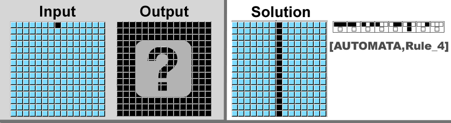
Even though the correct solution seems accessible, this is not really a good ARC-type puzzle. The puzzle should appear to have an intuitive answer. At this point, the reader will already be primed to expect an Elementary Cellular Automata. But the adjacent-pixel situation in the bottom row will nevertheless be baffling. Let's see if the next one is more intuitive.
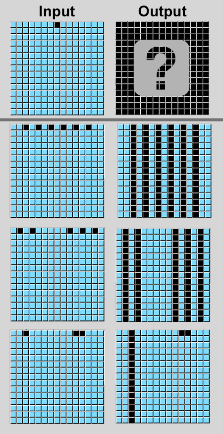
Not Intuitive
The first thing to note is that the input grids are identical to those in the previous puzzle. Even though I am familiar with the various ECA patterns, the output grids don't give me a sense of which rule to apply. ARCHIE on the other hand, compares the Inputs and Outputs and readily recognizes this as an ECA based puzzle and the ECA Rule that generates each output.
Now knowing that Rule 18 generated these latest example patterns, you might scroll back up in the article and look at a larger Rule 18 illustration. In comparison, the solution grid appears truncated halfway down, but that is where the first large triangle would appear within a larger grid. So another lesson is that the patterns depend on the ECA Rule, the originating rows, and the size constraints of the grid.
Better or Worse?
This puzzle is not only more inscrutable than the previous one, it is NOTABLE for this feature. This is Rule 30. By ARC Puzzle standards, the Rule 30 puzzle might be the hardest possible. The pattern generated by Rule 30 meets the rigorous definition of chaos and displays sensitive dependence on initial conditions. Stephen Wolfram used the center column of cells as a pseudorandom number generator for his program Mathematica. This means that unless you've figured out that the pattern came from the Rule 30 ECA, it should be impossible to solve. Rule 30 is a prime example of how complex behavior can emerge from simple rules.
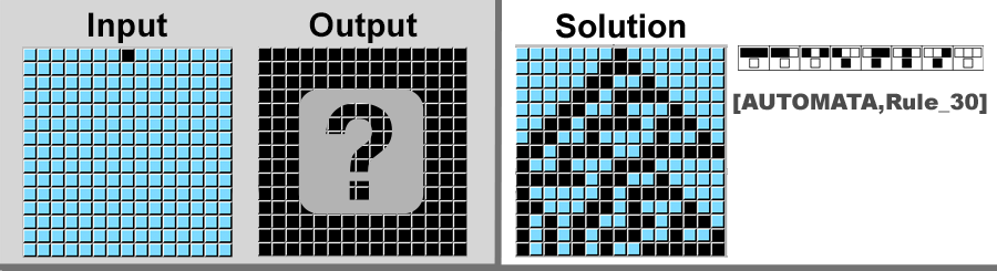
Let's backtrack for a moment and investigate a brute-force way to solve a puzzle like this. The grid is 15x15 or 225 total pixels. Each pixel can have a color value from 0 to 9, just like our counting numbers. But this means there are 10225 possible arrangements for this grid. You could never match known patterns within the time frame of the known universe. And yet ARCHIE solves this puzzle as easily as our first Rule 4 puzzle.
After exhausting the behavior of the 256 possible Elementary Cellular Automata, Stephen Wolfram began exploring more complicated rule sets. But he didn't jump straight to ARCHIE's neighborhood of 8 pixels with 10 states each. Instead, Wolfram simply added a third grey pixel to the standard black-and-white. Shockingly, with this minimal change, the number of possible rules jumps from 256 to 7,625,597,484,987. Wow2.
What Wolfram found with this and other massive rule sets is that a pseudorandom pattern like Rule 30 occurs less than 1% of the time.
It took far less time to "train" ARCHIE to solve the Rule 4 puzzle (single pixel to vertical line) than to create the graphics explaining it. "Train" is really the wrong term, as it echoes the way probabilistic neural networks need to develop capabilities: A galaxy of examples combined with statistical inference. I think you could feed any of the supposed AGI models an unlimited number of Rule 4 configurations, and they would never abstract their way to solving Rule 30.
I "showed" ARCHIE how to solve Rule 4 in a way very similar to how I would extend a person's understanding of ECAs. It did this by adding code explaining how Wolfram's numbering scheme worked: Wolfram's Rule number in decimal is converted to binary, and the 1s indicate where the next object pixel will be placed. Scan the grid left to right and populate down the rows. The "ECA Neighborhood" ARCHIE needs to scan is far less demanding than normal. And ARCHIE is already determining which pixels are objects against the detected background.
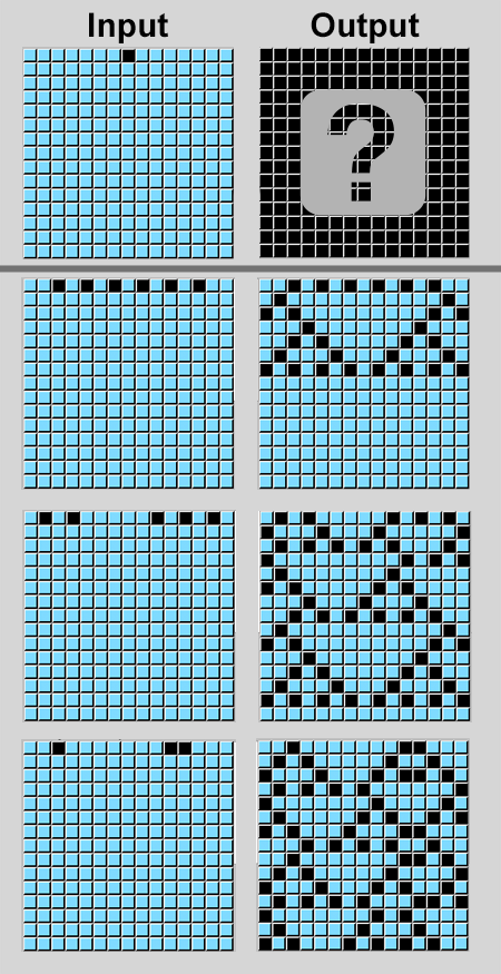
One Last Example to Demonstrate Abstraction
For ARCHIE, grid sizes and colors are already abstract notions across hundreds of puzzle types.
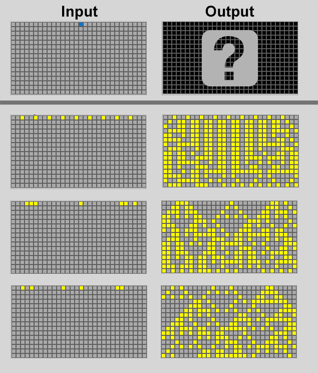
The background color is different than previous ECA Puzzles, and so are the grid dimensions. Example cell colors are different (yellow) from before, and the test cell color (blue) is different from any example. And yet, armed with the capability of solving the original Rule 4, ARCHIE's abstraction capabilities can detect and replicate the fractal pattern of the Rule 90 Sierpiński Triangle.
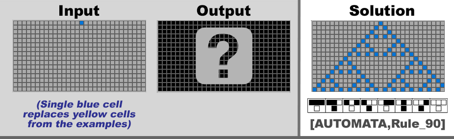
This is yet another example of how ARCHIE's Classic AI approach continues to tackle ever harder problems while reducing the need for additional resources.
To provide an analogy, ARCHIE has evolved into a Problem-Solving Framework, and these difficult puzzle types simply require "plug-in" additions. There is no "trial and error" path to success at this level. This is the way human problem-solving advances.
You can leave thoughtful comments or questions at the link below.
1. Stephen Wolfram - 2002, "A New Kind of Science" The full book is available for free online and is an invaluable study of Cellular Automata and their importance.
2. The formula is #_Rules = #_Results(#_Configurations).
Considering only three cells across the top, which can each have 2 states (black or white), there are 23 or 8 possible Configurations. Each of these configurations can yield one of two Results, a black or white cell. 28 is 256 possible "Rules."
Adding a third "grey" state for a cell yield 33 = 27 Configurations across the top. The third type of Result (black, white, grey) yields 327 i.e. 7,625,597,484,987 Rules. That is such a crazy jump from 256 that I had to do this math to confirm it!